 Webscraping, eBird, and Shiny with rebird
- 13 mins What is eBird?

eBird is an online database of bird observations that are crowdsourced by citizen scientists. Citizen science at its core is public participation in scientific research. Using either an app or the web interface, users input data about the species of bird they encountered, the count, location, and other metadata from their outings. eBird is widely used by the birding community and provides hundreds of millions of observations each year! This data provides real time insight into bird abundance and distribution at several spatial and temporal scales.
As a lover of birds myself, and an occasional user of eBird, I thought that this would be an excellent source of data for some fun visualizations.
I made a Shiny!
A couple years back I created a Shiny application that was focused on eBird data. It was a fun project that implemented:
CHECK IT OUT HERE!
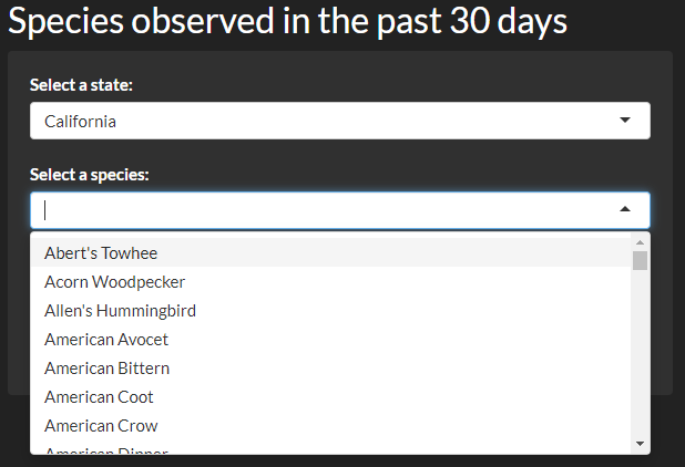
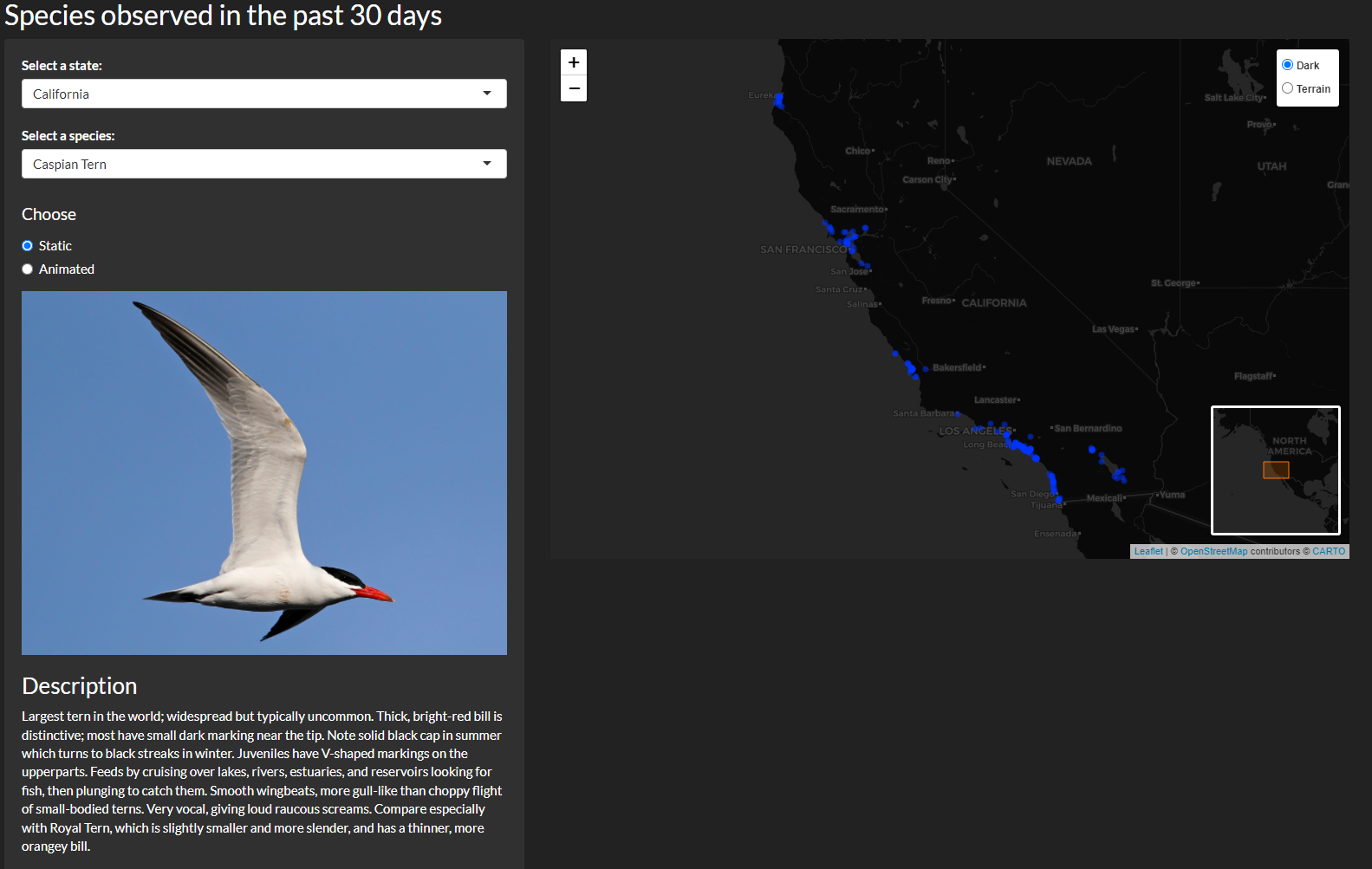
You can visualize observations on a map for each state for each species of bird that has been observed by eBird in the past 30 days. It provides an image of the select species, a description, and also lets you visualize an animation of observations over that 30 day period. The second tab Notables Nearby takes your location, and identifies locations that have had notable species sightings recently. Notable species are those that are rare or uncommon in the region.
Let’s break it down
Step 1. Get some data
In order to get eBird data, I used the package rebird which serves as an R interface with the eBird database. Using rebird requires attaining and providing an API key which is linked an eBird account, which can be done here. Once that is set up, you’ll be set up to get taxonomic data and most importantly observation data (up to 30 days).
Function usage
library(rebird)

EBIRD_KEY <- "YOUR_API_KEY_HERE"
species_code()
All rebird functions require a species code. This can be retrieved by using species_code() and supplying the scientific name.
species_code('hydroprogne caspia')

# "caster1"
ebirdtaxonomy()
ebirdtaxonomy() can be used to retrieve a dataframe of all the possible taxa in the eBird taxonomy. Here you will be able to see the possible common names, scientific names, species codes, and other various metadata.
tax <- rebird::ebirdtaxonomy()
head(tax)

# # A tibble: 6 x 15
# sciName    comName  speciesCode category taxonOrder bandingCodes comNameCodes sciNameCodes order
# <chr>      <chr>    <chr>       <chr>         <dbl> <chr>        <chr>        <chr>        <chr>
#   1 Struthio ~ Common ~ ostric2     species           1 NA           COOS         STCA         Stru~
#   2 Struthio ~ Somali ~ ostric3     species           6 NA           SOOS         STMO         Stru~
#   3 Struthio ~ Common/~ y00934      slash             7 NA           SOOS,COOS    STCA,STMO    Stru~
#   4 Rhea amer~ Greater~ grerhe1     species           8 NA           GRRH         RHAM         Rhei~
#   5 Rhea penn~ Lesser ~ lesrhe2     species          14 NA           LERH         RHPE         Rhei~
#   6 Rhea penn~ Lesser ~ lesrhe4     issf             15 NA           LERH,LR      RHPE         Rhei~
#   # ... with 6 more variables: familyCode <chr>, familyComName <chr>, familySciName <chr>,
#   #   reportAs <chr>, extinct <lgl>, extinctYear <int>
ebirdregion()
ebirdregion() returns the most recent sighting information reported in a given region or hotspot. You can also supply a number of days back to retrieve with a maximum of 30 days. Optionally, you may provide a single species code to retrieve observations for.
ebirdregion(loc = 'US-CA', key = EBIRD_KEY, back = 5)

# # A tibble: 374 x 13
# speciesCode comName   sciName   locId locName     obsDt howMany   lat   lng obsValid
# <chr>       <chr>     <chr>     <chr> <chr>       <chr>   <int> <dbl> <dbl> <lgl>
#   1 oaktit      Oak Titm~ Baeoloph~ L160~ Ninth & He~ 2022~       1  37.9 -122. TRUE
# 2 whcspa      White-cr~ Zonotric~ L160~ Ninth & He~ 2022~       1  37.9 -122. TRUE
# 3 houfin      House Fi~ Haemorho~ L160~ Ninth & He~ 2022~       3  37.9 -122. TRUE
# 4 yerwar      Yellow-r~ Setophag~ L160~ Ninth & He~ 2022~       2  37.9 -122. TRUE
# 5 amecro      American~ Corvus b~ L160~ Ninth & He~ 2022~       1  37.9 -122. TRUE
# 6 normoc      Northern~ Mimus po~ L160~ Ninth & He~ 2022~       2  37.9 -122. TRUE
# 7 lesgol      Lesser G~ Spinus p~ L160~ Ninth & He~ 2022~       1  37.9 -122. TRUE
# 8 moudov      Mourning~ Zenaida ~ L160~ Ninth & He~ 2022~       2  37.9 -122. TRUE
# 9 bewwre      Bewick's~ Thryoman~ L160~ Ninth & He~ 2022~       3  37.9 -122. TRUE
# 10 annhum      Anna's H~ Calypte ~ L141~ 40525 Hidd~ 2022~       2  37.3 -120. TRUE
ebirdnotable()
ebirdnotable() returns the most recent notable observations given either a latitude/longitude, hotspot, location ID, or region.
ebirdnotable(lat = 36.96, lng = -122.01, dist = 15, key = EBIRD_KEY)

# # A tibble: 50 x 13
# speciesCode comName   sciName    locId  locName       obsDt  howMany   lat   lng obsValid obsReviewed
# <chr>       <chr>     <chr>      <chr>  <chr>         <chr>    <int> <dbl> <dbl> <lgl>    <lgl>
#   1 lucwar      Lucy's W~ Leiothlyp~ L1336~ Tyrrell Park  2022-~       1  37.0 -122. FALSE    FALSE
#  2 naswar      Nashvill~ Leiothlyp~ L1229~ Kenneth Stre~ 2022-~       1  37.0 -122. FALSE    FALSE
#  3 lawgol      Lawrence~ Spinus la~ L1336~ Tyrrell Park  2022-~       1  37.0 -122. FALSE    FALSE
#  4 lawgol      Lawrence~ Spinus la~ L1336~ Tyrrell Park  2022-~       1  37.0 -122. FALSE    FALSE
#  5 lawgol      Lawrence~ Spinus la~ L1336~ Tyrrell Park  2022-~       1  37.0 -122. FALSE    FALSE
#  6 naswar      Nashvill~ Leiothlyp~ L1229~ Kenneth Stre~ 2022-~       1  37.0 -122. TRUE     TRUE
#  7 foxsp1      Fox Spar~ Passerell~ L1180~ 3777 Cherryv~ 2022-~       1  37.0 -122. TRUE     TRUE
#  8 trokin      Tropical~ Tyrannus ~ L6273~ San Lorenzo ~ 2022-~       1  37.0 -122. TRUE     TRUE
#  9 lucwar      Lucy's W~ Leiothlyp~ L1336~ Tyrrell Park  2022-~       1  37.0 -122. TRUE     TRUE
# 10 lucwar      Lucy's W~ Leiothlyp~ L1336~ Tyrrell Park  2022-~       1  37.0 -122. TRUE     TRUE
# # ... with 40 more rows, and 2 more variables: locationPrivate <lgl>, subId <chr>
Step 2. Map the data
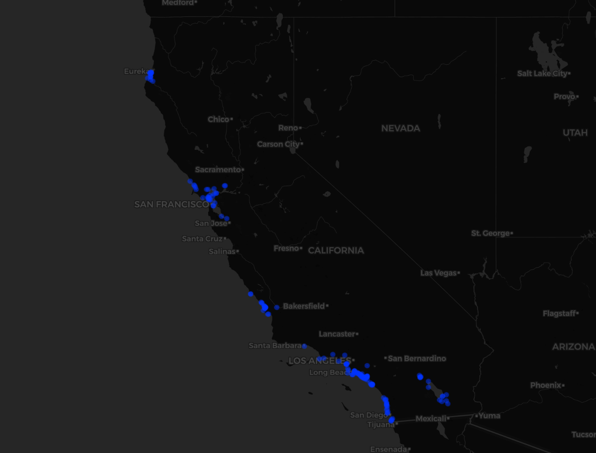
Here I will show a simple example of how to retrieve observation data for a single species, and visualize it on a map using leaflet. I will map observations in the past 30 days for Caspian Terns in California.
# Find the species code for Caspian Tern
tax$speciesCode[tax$comName == 'Caspian Tern']

# "caster1"

# Get observations in past 30 days in California
cate <- ebirdregion(loc = 'US-CA',
                    species = 'caster1',
                    key = EBIRD_KEY,
                    back = 30)

# Map it!
leaflet(data = cate) %>%
  addProviderTiles(provider = providers$CartoDB.DarkMatter) %>%
  addCircleMarkers(~lng, ~lat,
                   popup = ~as.character(locName),
                   label = ~as.character(locName),
                   radius = 1)
And voila, here is what the map looks like!
Step 3. Add reactivity for Shiny
The beauty of Shiny to me is the reactivity. A user selects or provides an input and the Shiny app reacts, and provides new data or visuals. I wanted to allow users to select a state of their choice and have a drop down menu of all the possible bird species that could be mapped with the common names rather than scientific names. The steps to accomplish this were:
- User provides state name
- Convert state name to region code (ex: California = CA)
- Retrieve observations for the provided state
- Get a unique list of species from the observations
- Return the list as common names
regionCodes <- ebirdsubregionlist("subnational1", "US", key = EBIRD_KEY)

head(regionCodes)

# # A tibble: 6 x 2
# code  name
# <chr> <chr>
#   1 US-AL Alabama
# 2 US-AK Alaska
# 3 US-AZ Arizona
# 4 US-AR Arkansas
# 5 US-CA California
# 6 US-CO Colorado
# User input here
stateInput <- 'California'
# Convert state name to region code
regionCode <- regionCodes %>%
filter(name == stateInput) %>%
pull(code)
# Get observations in past 30 days in California
obs <- ebirdregion(loc = regionCode, key = EBIRD_KEY, back = 30)
# Unique bird common names
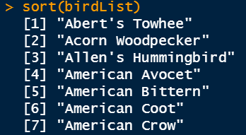
birdList <- unique(obs$comName)
Step 4. Webscrape to add species pictures and descriptions!
To add dynamic photos and descriptions to the user’s species selection I used the webscraping package rvest which is conveniently part of the tidyverse! I realized that because rebird utilizes species codes, and that the eBird site has a species profile that is easily organized by the species code in the url, I could easily scrape images and descriptions for individual bird.
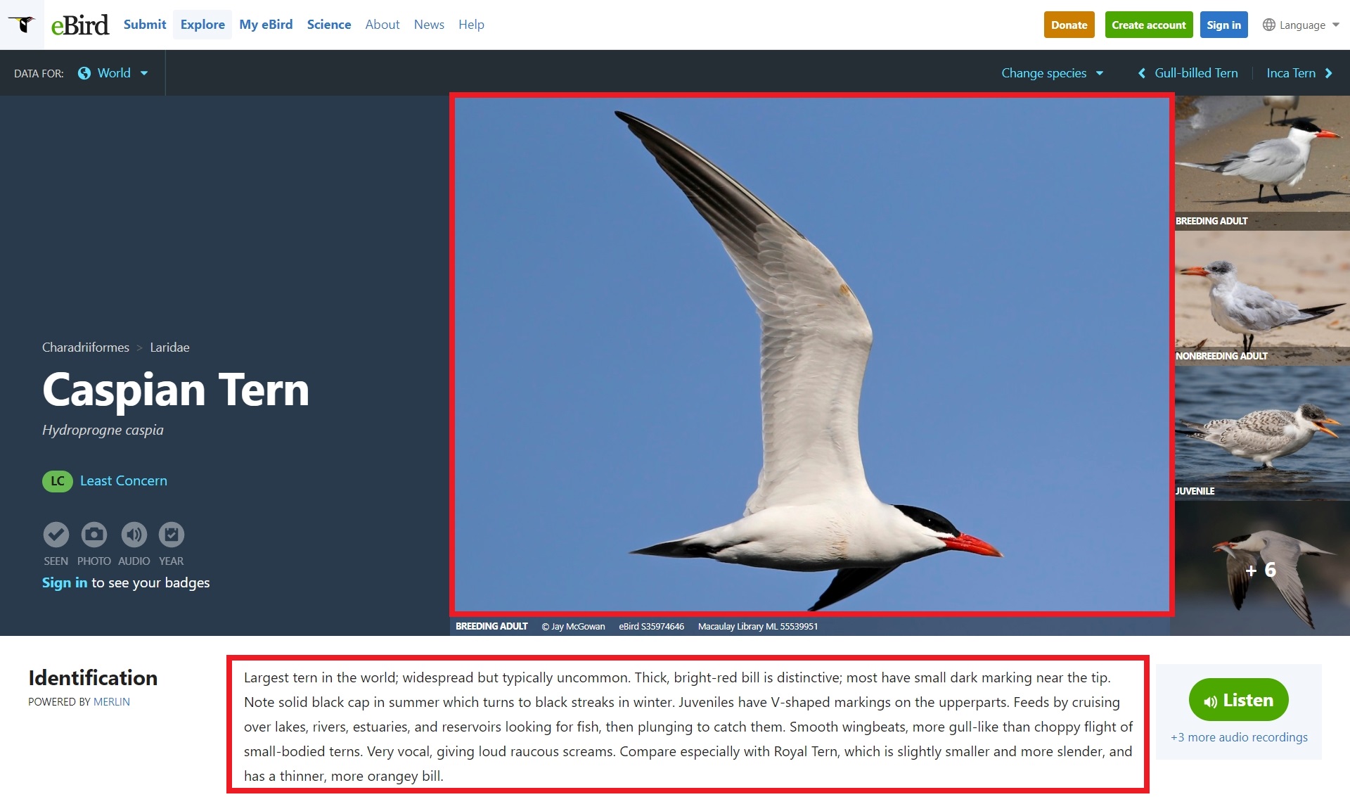
Here is a species profile page for Caspian Tern. Notice that the species code caster1 is used in the url. This allows me to easily manipulate the url to grab information for specific birds.
https://ebird.org/species/caster1
Now let’s grab the image and the description.
# Build the url for a species providing the species code
speciesCode <- "caster1"
url <- paste0("https://ebird.org/species/", speciesCode)

# Use rvest to read the html of the url provide
imgsrc <- read_html(url) %>%
  # html_node finds the HTML tags
  html_node(xpath = '//*/img') %>%
  # html_attr returns the attribute
  html_attr('src')

imgsrc

# "https://cdn.download.ams.birds.cornell.edu/api/v1/asset/308395131/1200"
# Get list of metatag tags
metatags <- read_html(url) %>%
  html_nodes('meta') %>%
  html_attr('name')

# > metatags
# [1] NA                         "copyright"                NA
# [4] "google-site-verification" "viewport"                 "msapplication-TileColor"
# [7] "msapplication-TileImage"  "theme-color"              "description"
# [10] NA                         NA                         NA
# [13] NA                         NA                         "twitter:card"
# [16] "twitter:site"


# Find which row has the description
rownum <- which(metatags == "description")

# > rownum
# [1] 9

# Grab the content
content <- read_html(url) %>%
  html_nodes('meta') %>%
  html_attr('content')

# Just the description content
content[rownum]

# > content[rownum]
# [1] "Largest tern in the world; widespread but typically uncommon. Thick,
# bright-red bill is distinctive; most have small dark marking near the tip.
# Note solid black cap in summer which turns to black streaks in winter.
# Juveniles have V-shaped markings on the upperparts. Feeds by cruising over
# lakes, rivers, estuaries, and reservoirs looking for fish, then plunging to
# catch them. Smooth  wingbeats, more gull-like than choppy flight of
# small-bodied terns. Very vocal, giving loud raucous screams. Compare
# especially with Royal Tern, which is slightly smaller and more slender, and
# has a thinner, more orangey bill.\n\r\n"
Putting it all together!
Thanks for reading! You can see the app in its entirety here.
Related Posts

Tom Pham
COVID-19 Data Analyst